Scalar, 1D{1} datasets
The 1D{1} datasets are one dimensional, \(d=1\), with one single-component, \(p=1\), dependent variable. In this section, we walk through some examples of 1D{1} datasets.
Let’s start by first importing the csdmpy module.
>>> import csdmpy as cp
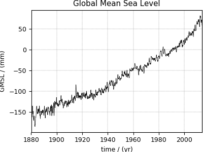
Global Mean Sea Level rise dataset
The following dataset is the Global Mean Sea Level (GMSL) rise from the late 19th to the Early 21st Century. The original dataset was downloaded as a CSV file and subsequently converted to the CSD model format. Let’s import this file.
>>> filename = 'Test Files/gmsl/GMSL.csdf'
>>> sea_level = cp.load(filename)
The variable filename is a string with the address to the sea_level.csdf
file.
The load() method of the csdmpy module reads the
file and returns an instance of the CSDM class, in
this case, as a variable sea_level. For a quick preview of the data
structure, use the data_structure attribute of this
instance.
>>> print(sea_level.data_structure)
{
  "csdm": {
    "version": "1.0",
    "read_only": true,
    "timestamp": "2019-05-21T13:43:00Z",
    "tags": [
      "Jason-2",
      "satellite altimetry",
      "mean sea level",
      "climate"
    ],
    "description": "Global Mean Sea Level (GMSL) rise from the late 19th to the Early 21st Century.",
    "dimensions": [
      {
        "type": "linear",
        "count": 1608,
        "increment": "0.08333333333 yr",
        "coordinates_offset": "1880.0416666667 yr",
        "quantity_name": "time",
        "reciprocal": {
          "quantity_name": "frequency"
        }
      }
    ],
    "dependent_variables": [
      {
        "type": "internal",
        "name": "Global Mean Sea Level",
        "unit": "mm",
        "quantity_name": "length",
        "numeric_type": "float32",
        "quantity_type": "scalar",
        "component_labels": [
          "GMSL"
        ],
        "components": [
          [
            "-183.0, -171.125, ..., 59.6875, 58.5"
          ]
        ]
      }
    ]
  }
}
Warning
The serialized string from the data_structure
attribute is not the same as the JSON serialization on the file.
This attribute is only intended for a quick preview of the data
structure and avoids displaying large datasets. Do not use
the value of this attribute to save the data to the file. Instead, use the
save() method of the CSDM
class.
The tuples of the dimensions and dependent variables from this example are
>>> x = sea_level.dimensions
>>> y = sea_level.dependent_variables
respectively. The coordinates along the dimension and the component of the dependent variable are
>>> print(x[0].coordinates)
[1880.04166667 1880.125      1880.20833333 ... 2013.79166666 2013.87499999
 2013.95833333] yr

>>> print(y[0].components[0])
[-183.     -171.125  -164.25   ...   66.375    59.6875   58.5   ]
respectively.
Tip
Plotting a one-dimension scalar line-plot.
Before we plot this dataset, we find it convenient to write a small plotting method. This method makes it easier, later, when we describe 1D{1} examples form a variety of scientific datasets. The method follows-
>>> import matplotlib.pyplot as plt
>>> def plot1D(dataObject):
...     # tuples of dependent and dimension instances.
...     x = dataObject.dimensions
...     y = dataObject.dependent_variables
...
...     plt.figure(figsize=(4,3))
...     plt.plot(x[0].coordinates, y[0].components[0].real, color='k', linewidth=0.5)
...
...     plt.xlim(x[0].coordinates[0].value, x[0].coordinates[-1].value)
...
...     # The axes labels and figure title.
...     plt.xlabel(x[0].axis_label)
...     plt.ylabel(y[0].axis_label[0])
...     plt.title(y[0].name)
...
...     plt.grid(color='gray', linestyle='--', linewidth=0.3)
...     plt.tight_layout(pad=0, w_pad=0, h_pad=0)
...     plt.show()
A quick walk-through of the plot1D method. The method accepts an
instance of the CSDM class as an argument. Within the method, we
make use of the instance’s attributes in addition to the matplotlib
functions. The first line assigns the tuple of the dimensions and dependent
variables to x and y, respectively. The following two lines add a plot of
the components of the dependent variable versus the coordinates of the dimension.
The next line sets the x-range. For labeling the axes,
we use the axis_label attribute
of both dimension and dependent variable instances. For the figure title,
we use the name attribute
of the dependent variable instance. The next statement adds the grid lines.
For additional information, refer to Matplotlib
documentation.
The plot1D method is only for illustrative purposes. The users may use any
plotting library to visualize their datasets.
Now to plot the sea_level dataset.
>>> plot1D(sea_level)
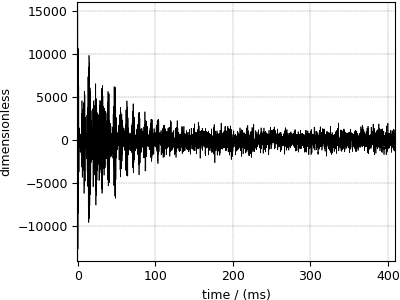
Nuclear Magnetic Resonance (NMR) dataset
The following dataset is a \(^{13}\mathrm{C}\) time-domain NMR Bloch decay signal of ethanol. Let’s load this data file and take a quick look at its data structure. We follow the previously described steps.
>>> filename = 'Test Files/NMR/blochDecay/blochDecay.csdf'
>>> NMR_data = cp.load(filename)
>>> print(NMR_data.data_structure)
{
  "csdm": {
    "version": "1.0",
    "read_only": true,
    "timestamp": "2016-03-12T16:41:00Z",
    "geographic_coordinate": {
      "altitude": "238.9719543457031 m",
      "longitude": "-83.05154573892345 °",
      "latitude": "39.97968794964322 °"
    },
    "tags": [
      "13C",
      "NMR",
      "spectrum",
      "ethanol"
    ],
    "description": "A time domain NMR 13C Bloch decay signal of ethanol.",
    "dimensions": [
      {
        "type": "linear",
        "count": 4096,
        "increment": "0.1 ms",
        "coordinates_offset": "-0.3 ms",
        "quantity_name": "time",
        "reciprocal": {
          "coordinates_offset": "-3005.363 Hz",
          "origin_offset": "75426328.86 Hz",
          "quantity_name": "frequency",
          "label": "13C frequency shift"
        }
      }
    ],
    "dependent_variables": [
      {
        "type": "internal",
        "numeric_type": "complex128",
        "quantity_type": "scalar",
        "components": [
          [
            "(-8899.40625-1276.7734375j), (-4606.88037109375-742.4124755859375j), ..., (37.548492431640625+20.156890869140625j), (-193.9228515625-67.06524658203125j)"
          ]
        ]
      }
    ]
  }
}
This particular example illustrates two additional attributes of the CSD model,
namely, the geographic_coordinate and
tags. The geographic_coordinate described the
location where the CSDM file was last serialized. You may access this
attribute through,
>>> NMR_data.geographic_coordinate
{'altitude': '238.9719543457031 m', 'longitude': '-83.05154573892345 °', 'latitude': '39.97968794964322 °'}
Similarly, the tags attribute can be accessed through,
>>> NMR_data.tags
['13C', 'NMR', 'spectrum', 'ethanol']
You may add additional tags, if so desired, to this list using the append method of python’s list class, such as
>>> NMR_data.tags.append("Bloch decay")
>>> NMR_data.tags
['13C', 'NMR', 'spectrum', 'ethanol', 'Bloch decay']
Unlike the previous example, the data structure of the NMR measurement is a complex-valued dependent variable where the values are
>>> y = NMR_data.dependent_variables
>>> print(y[0].components[0])
[-8899.40625   -1276.7734375j  -4606.88037109 -742.41247559j
  9486.43847656 -770.0413208j  ...   -70.95385742  -28.32843018j
    37.54849243  +20.15689087j  -193.92285156  -67.06524658j]
The coordinates along the dimension are
>>> x = NMR_data.dimensions
>>> x0 = x[0].coordinates
>>> print(x0)
[-3.000e-01 -2.000e-01 -1.000e-01 ...  4.090e+02  4.091e+02  4.092e+02] ms
Now to the plot the dataset,
>>> plot1D(NMR_data)
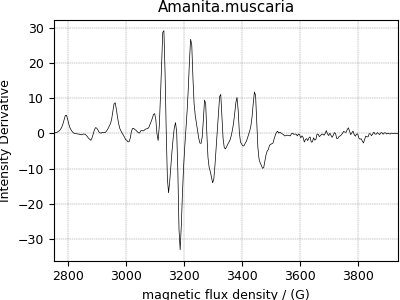
Electron Paramagnetic Resonance (EPR) dataset
The following simulation of the EPR dataset is formerly obtained as a JCAMP-DX file and subsequently converted to the CSD model file-format. The data structure of this dataset and the corresponding plot follows,
>>> filename = 'Test Files/EPR/AmanitaMuscaria_base64.csdf'
>>> EPR_data = cp.load(filename)
>>> print(EPR_data.data_structure)
{
  "csdm": {
    "version": "1.0",
    "read_only": true,
    "timestamp": "2015-02-26T16:41:00Z",
    "description": "A Electron Paramagnetic Resonance simulated dataset.",
    "dimensions": [
      {
        "type": "linear",
        "count": 298,
        "increment": "4.0 G",
        "coordinates_offset": "2750.0 G",
        "quantity_name": "magnetic flux density"
      }
    ],
    "dependent_variables": [
      {
        "type": "internal",
        "name": "Amanita.muscaria",
        "numeric_type": "float32",
        "quantity_type": "scalar",
        "component_labels": [
          "Intensity Derivative"
        ],
        "components": [
          [
            "0.067, 0.136, ..., -0.035, -0.137"
          ]
        ]
      }
    ]
  }
}
>>> plot1D(EPR_data)
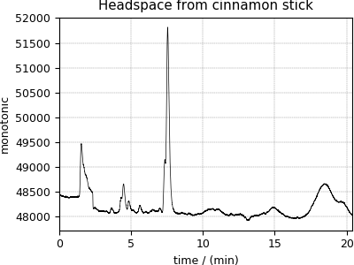
Gas Chromatography dataset
The following Gas Chromatography dataset is also obtained as a JCAMP-DX file and subsequently converted to the CSD model file-format. The data structure and the plot of the gas chromatography dataset follows,
>>> filename = 'Test Files/GC/cinnamon_none.csdf'
>>> GCData = cp.load(filename)
>>> print(GCData.data_structure)
{
  "csdm": {
    "version": "1.0",
    "read_only": true,
    "timestamp": "2011-12-16T12:24:10Z",
    "description": "A Gas Chromatography dataset of cinnamon stick.",
    "dimensions": [
      {
        "type": "linear",
        "count": 6001,
        "increment": "0.0034 min",
        "quantity_name": "time",
        "reciprocal": {
          "quantity_name": "frequency"
        }
      }
    ],
    "dependent_variables": [
      {
        "type": "internal",
        "name": "Headspace from cinnamon stick",
        "numeric_type": "float32",
        "quantity_type": "scalar",
        "component_labels": [
          "monotonic"
        ],
        "components": [
          [
            "48453.0, 48444.0, ..., 48040.0, 48040.0"
          ]
        ]
      }
    ]
  }
}
>>> plot1D(GCData)
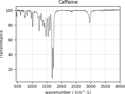
Fourier Transform Infrared Spectroscopy (FTIR) dataset
For the following FTIR dataset, we again convert the original JCAMP-DX file to the CSD model file-format. The data structure and the plot of the FTIR dataset follows,
>>> filename = 'Test Files/IR/caffeine_none.csdf'
>>> FTIR_data = cp.load(filename)
>>> print(FTIR_data.data_structure)
{
  "csdm": {
    "version": "1.0",
    "read_only": true,
    "timestamp": "2019-07-01T21:03:42Z",
    "description": "An IR spectrum of caffeine.",
    "dimensions": [
      {
        "type": "linear",
        "count": 1842,
        "increment": "1.930548614883216 cm^-1",
        "coordinates_offset": "449.41 cm^-1",
        "quantity_name": "wavenumber",
        "reciprocal": {
          "quantity_name": "length"
        }
      }
    ],
    "dependent_variables": [
      {
        "type": "internal",
        "name": "Caffeine",
        "numeric_type": "float32",
        "quantity_type": "scalar",
        "component_labels": [
          "Transmittance"
        ],
        "components": [
          [
            "99.31053, 99.08212, ..., 100.22944, 100.22944"
          ]
        ]
      }
    ]
  }
}
>>> plot1D(FTIR_data)
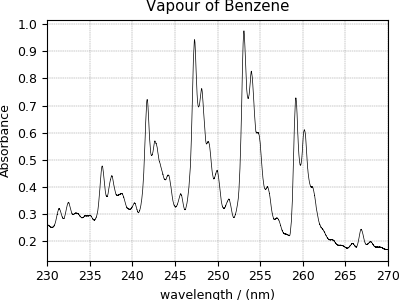
Ultraviolet–visible (UV-vis) dataset
The following UV-vis dataset is originally downloaded as a JCAMP-DX file and consequently turned to the CSD model file-format. The data structure and the plot of the UV-vis dataset follows,
>>> filename = 'Test Files/UV-Vis/benzeneVapour_base64.csdf'
>>> UV_data = cp.load(filename)
>>> print(UV_data.data_structure)
{
  "csdm": {
    "version": "1.0",
    "read_only": true,
    "timestamp": "2014-09-30T11:16:33Z",
    "description": "A UV-vis spectra of benzene vapours.",
    "dimensions": [
      {
        "type": "linear",
        "count": 4001,
        "increment": "0.01 nm",
        "coordinates_offset": "230.0 nm",
        "quantity_name": "length",
        "label": "wavelength",
        "reciprocal": {
          "quantity_name": "wavenumber"
        }
      }
    ],
    "dependent_variables": [
      {
        "type": "internal",
        "name": "Vapour of Benzene",
        "numeric_type": "float32",
        "quantity_type": "scalar",
        "component_labels": [
          "Absorbance"
        ],
        "components": [
          [
            "0.25890622, 0.25923702, ..., 0.16814752, 0.16786034"
          ]
        ]
      }
    ]
  }
}
>>> plot1D(UV_data)
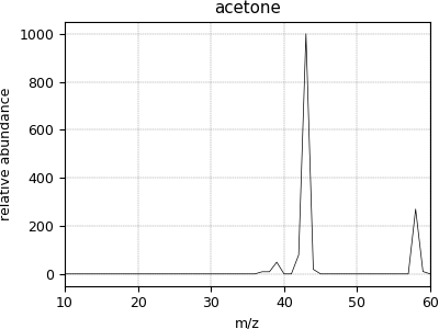
Mass spectrometry dataset
The following is an example of a sparse dataset. The acetone.csdf CSDM data file is stored as a sparse dependent variable data. Upon import, the values of the dependent variable component sparsely populate the coordinate grid. The remaining unpopulated coordinates are assigned a zero value.
>>> filename = 'Test Files/MassSpec/acetone.csdf'
>>> mass_spec = cp.load(filename)
>>> print(mass_spec.data_structure)
{
  "csdm": {
    "version": "1.0",
    "read_only": true,
    "timestamp": "2019-06-23T17:53:26Z",
    "description": "MASS spectrum of acetone",
    "dimensions": [
      {
        "type": "linear",
        "count": 51,
        "increment": "1.0",
        "coordinates_offset": "10.0",
        "label": "m/z"
      }
    ],
    "dependent_variables": [
      {
        "type": "internal",
        "name": "acetone",
        "numeric_type": "float32",
        "quantity_type": "scalar",
        "component_labels": [
          "relative abundance"
        ],
        "components": [
          [
            "0.0, 0.0, ..., 10.0, 0.0"
          ]
        ]
      }
    ]
  }
}
Here, the coordinates along the dimension are
>>> print(mass_spec.dimensions[0].coordinates)
[10. 11. 12. 13. 14. 15. 16. 17. 18. 19. 20. 21. 22. 23. 24. 25. 26. 27.
 28. 29. 30. 31. 32. 33. 34. 35. 36. 37. 38. 39. 40. 41. 42. 43. 44. 45.
 46. 47. 48. 49. 50. 51. 52. 53. 54. 55. 56. 57. 58. 59. 60.]
and the components of the dependent variable follow
>>> print(mass_spec.dependent_variables[0].components[0])
[   0.    0.    0.    0.    0.    0.    0.    0.    0.    0.    0.    0.
    0.    0.    0.    0.    0.    0.    0.    0.    0.    0.    0.    0.
    0.    0.    0.    9.    9.   49.    0.    0.   79. 1000.   19.    0.
    0.    0.    0.    0.    0.    0.    0.    0.    0.    0.    0.    0.
  270.   10.    0.]
Note, only eight values were specified in the dependent variable components attribute in the .csdf file. The remaining component values are set to zero.
Now to plot the dataset.
>>> plot1D(mass_spec)